I’d like to introduce you to the graph of $x=\sin(f_1t)e^{d_1t}$, $y=\sin(f_2t)e^{d_2t}$, a curve that spins, laughs and dances.

“But what is this witchcraft?” I hear you ask. Well, sit yourself down somewhere comfortable and I’ll tell you.

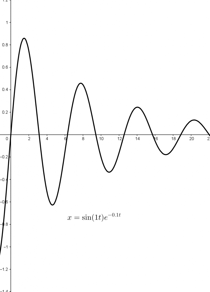
$x=\sin(f_1t)e^{d_1t}$, $y=\sin(f_2t)e^{d_2t}$ is a system of parametric equations, where $x$ and $y$ are each defined by a function in terms of $t$. The underlying functions look like this, for $f_1=f_2=1, d_1=d_2=0$.

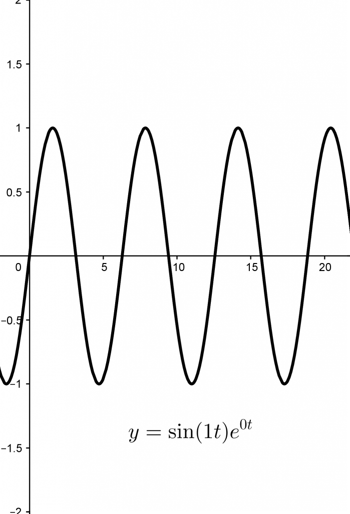
They’re just sine waves! And with these values of the variables the graph is, frankly, boring.

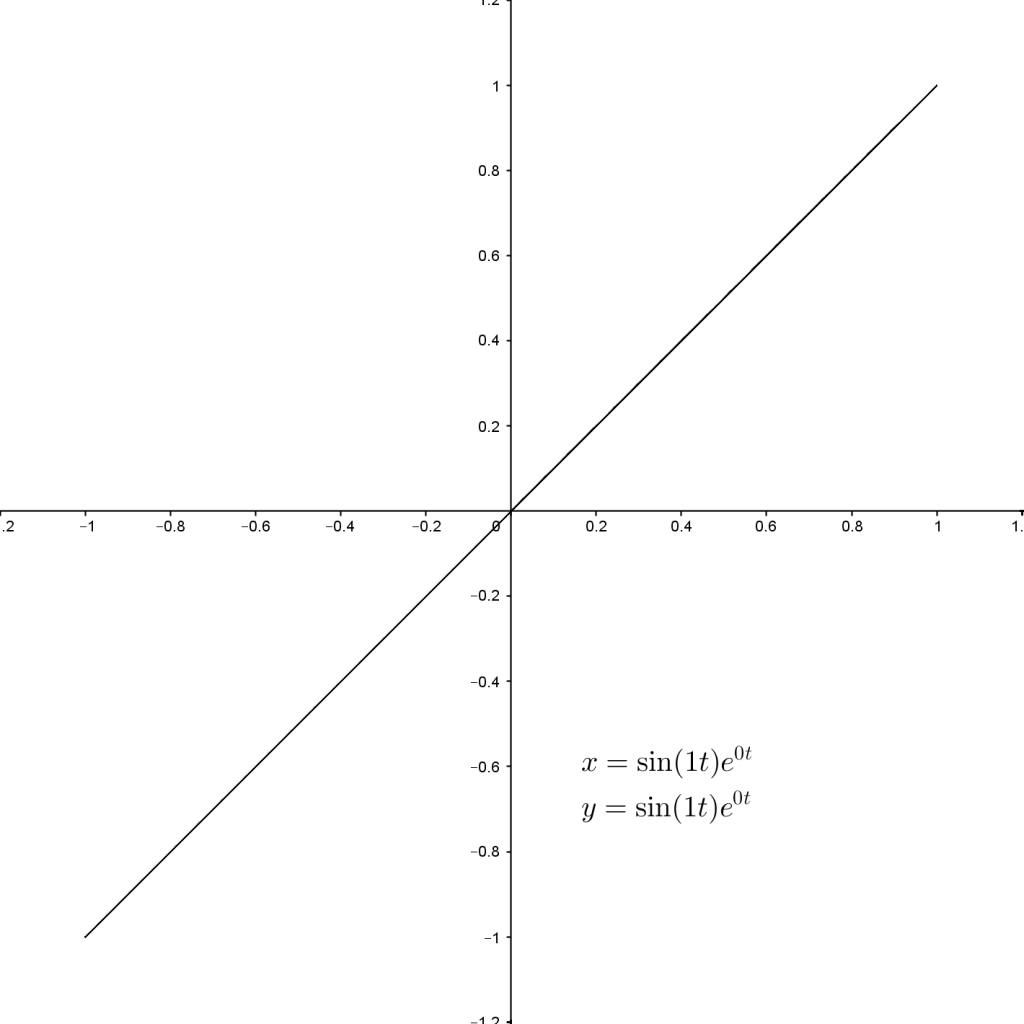
$x$ and $y$ have the same value for every value of $t$, so the graph of the parametric equations is the graph of $y=x$.

When $f_1$ and $f_2$ are different, things start to get more interesting.

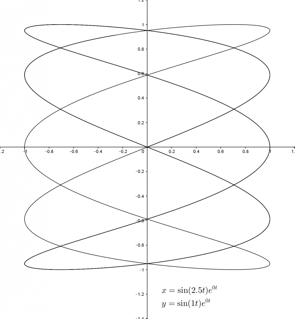
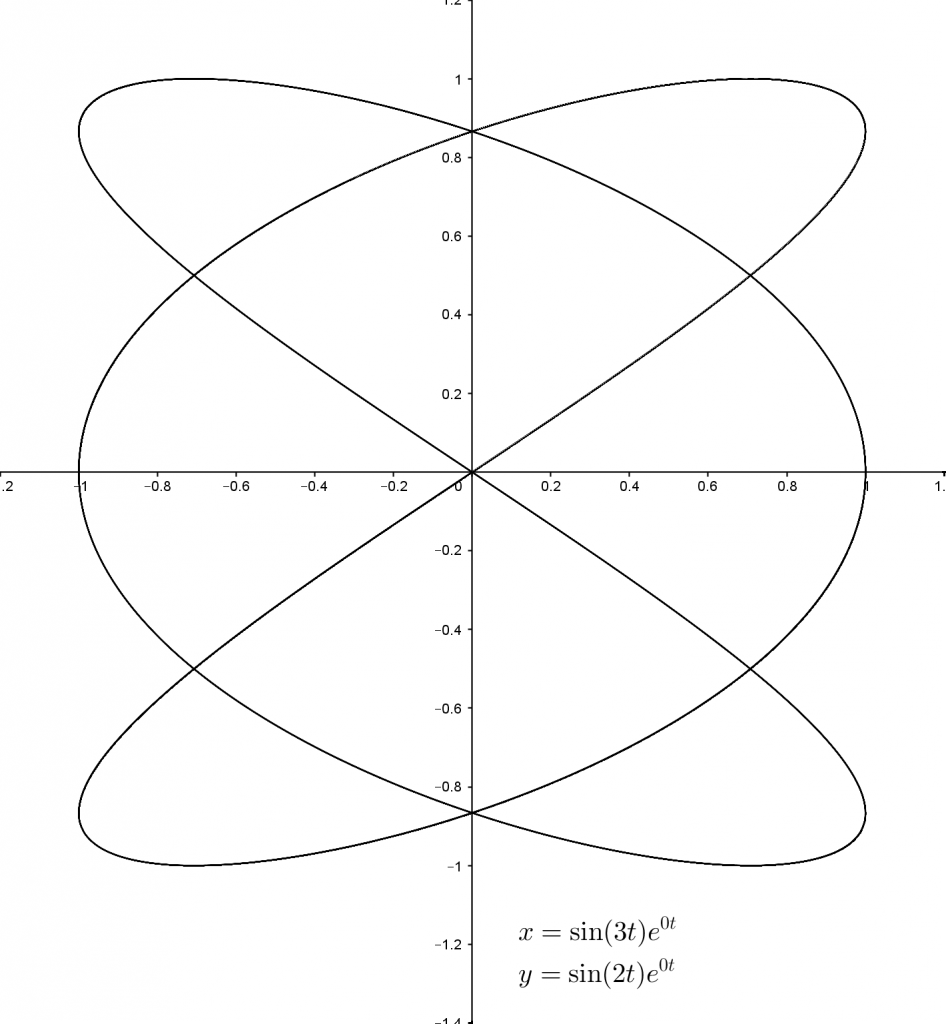
In this form the curves are known as Lissajous curves. But if we change $d_1$ and $d_2$ as well, things get even more interesting. Using negative values for these variables has the effect of dampening the underlying functions – the sine waves get smaller as $t$ gets bigger.

We could also use positive values for $d_1$ and $d_2$; this makes the sine waves get bigger as $t$ gets bigger, which has much the same effect on the final curve, although you might need to zoom out to see it.

Here are the graphs with the same $f_1$ and $f_2$ values as earlier, but with $d_1=d_2=-0.1$.

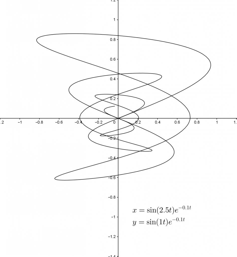
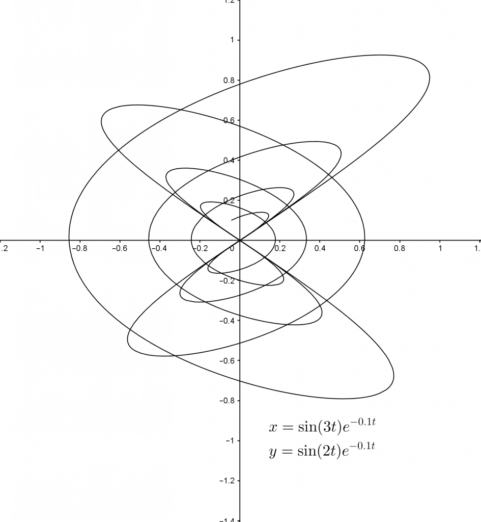
These curves are known as harmonograph curves. The name comes from a Victorian device consisting of two pendulums of different lengths swinging at right angles to each other, with a pencil suspended between them. As the pendulums swing, the pencil moves and draws a curve representing the combined movement of the pendulums, producing curves very much like the ones above.

In the interactive below you can try different values of $f_1$, $f_2$, $d_1$ and $d_2$. What glorious curves can you find? What effect does the ratio $f_1 : f_2$ have on the curve? What happens when $d_1$ and $d_2$ are different?